Testing hierarchical parent degradation kinetics with residue data on dimethenamid and dimethenamid-P
Johannes Ranke
Last change on 5 January 2023, last compiled on 12 Mai 2025
Source:vignettes/prebuilt/2022_dmta_parent.rmd
2022_dmta_parent.rmdIntroduction
The purpose of this document is to demonstrate how nonlinear hierarchical models (NLHM) based on the parent degradation models SFO, FOMC, DFOP and HS can be fitted with the mkin package.
It was assembled in the course of work package 1.1 of Project Number 173340 (Application of nonlinear hierarchical models to the kinetic evaluation of chemical degradation data) of the German Environment Agency carried out in 2022 and 2023.
The mkin package is used in version 1.2.10. It contains the test data
and the functions used in the evaluations. The saemix
package is used as a backend for fitting the NLHM, but is also loaded to
make the convergence plot function available.
This document is processed with the knitr package, which
also provides the kable function that is used to improve
the display of tabular data in R markdown documents. For parallel
processing, the parallel package is used.
library(mkin)
library(knitr)
library(saemix)
library(parallel)
n_cores <- detectCores()
if (Sys.info()["sysname"] == "Windows") {
  cl <- makePSOCKcluster(n_cores)
} else {
  cl <- makeForkCluster(n_cores)
}
Data
The test data are available in the mkin package as an object of class
mkindsg (mkin dataset group) under the identifier
dimethenamid_2018. The following preprocessing steps are
still necessary:
- The data available for the enantiomer dimethenamid-P (DMTAP) are renamed to have the same substance name as the data for the racemic mixture dimethenamid (DMTA). The reason for this is that no difference between their degradation behaviour was identified in the EU risk assessment.
- The data for transformation products and unnecessary columns are discarded
- The observation times of each dataset are multiplied with the corresponding normalisation factor also available in the dataset, in order to make it possible to describe all datasets with a single set of parameters that are independent of temperature
- Finally, datasets observed in the same soil (
Elliot 1andElliot 2) are combined, resulting in dimethenamid (DMTA) data from six soils.
The following commented R code performs this preprocessing.
# Apply a function to each of the seven datasets in the mkindsg object to create a list
dmta_ds <- lapply(1:7, function(i) {
  ds_i <- dimethenamid_2018$ds[[i]]$data                     # Get a dataset
  ds_i[ds_i$name == "DMTAP", "name"] <-  "DMTA"              # Rename DMTAP to DMTA
  ds_i <- subset(ds_i, name == "DMTA", c("name", "time", "value")) # Select data
  ds_i$time <- ds_i$time * dimethenamid_2018$f_time_norm[i]  # Normalise time
  ds_i                                                       # Return the dataset
})

# Use dataset titles as names for the list elements
names(dmta_ds) <- sapply(dimethenamid_2018$ds, function(ds) ds$title)

# Combine data for Elliot soil to obtain a named list with six elements
dmta_ds[["Elliot"]] <- rbind(dmta_ds[["Elliot 1"]], dmta_ds[["Elliot 2"]]) #
dmta_ds[["Elliot 1"]] <- NULL
dmta_ds[["Elliot 2"]] <- NULL
The following tables show the 6 datasets.
for (ds_name in names(dmta_ds)) {
    print(kable(mkin_long_to_wide(dmta_ds[[ds_name]]),
      caption = paste("Dataset", ds_name),
      label = paste0("tab:", ds_name), booktabs = TRUE))
    cat("\n\\clearpage\n")
}| time | DMTA |
|---|---|
| 0 | 95.8 |
| 0 | 98.7 |
| 14 | 60.5 |
| 30 | 39.1 |
| 59 | 15.2 |
| 120 | 4.8 |
| 120 | 4.6 |
| time | DMTA |
|---|---|
| 0.000000 | 100.5 |
| 0.000000 | 99.6 |
| 1.941295 | 91.9 |
| 1.941295 | 91.3 |
| 6.794534 | 81.8 |
| 6.794534 | 82.1 |
| 13.589067 | 69.1 |
| 13.589067 | 68.0 |
| 27.178135 | 51.4 |
| 27.178135 | 51.4 |
| 56.297565 | 27.6 |
| 56.297565 | 26.8 |
| 86.387643 | 15.7 |
| 86.387643 | 15.3 |
| 115.507073 | 7.9 |
| 115.507073 | 8.1 |
| time | DMTA |
|---|---|
| 0.0000000 | 96.5 |
| 0.0000000 | 96.8 |
| 0.0000000 | 97.0 |
| 0.6233856 | 82.9 |
| 0.6233856 | 86.7 |
| 0.6233856 | 87.4 |
| 1.8701567 | 72.8 |
| 1.8701567 | 69.9 |
| 1.8701567 | 71.9 |
| 4.3636989 | 51.4 |
| 4.3636989 | 52.9 |
| 4.3636989 | 48.6 |
| 8.7273979 | 28.5 |
| 8.7273979 | 27.3 |
| 8.7273979 | 27.5 |
| 13.0910968 | 14.8 |
| 13.0910968 | 13.4 |
| 13.0910968 | 14.4 |
| 17.4547957 | 7.7 |
| 17.4547957 | 7.3 |
| 17.4547957 | 8.1 |
| 26.1821936 | 2.0 |
| 26.1821936 | 1.5 |
| 26.1821936 | 1.9 |
| 34.9095915 | 1.3 |
| 34.9095915 | 1.0 |
| 34.9095915 | 1.1 |
| 43.6369893 | 0.9 |
| 43.6369893 | 0.7 |
| 43.6369893 | 0.7 |
| 52.3643872 | 0.6 |
| 52.3643872 | 0.4 |
| 52.3643872 | 0.5 |
| 74.8062674 | 0.4 |
| 74.8062674 | 0.3 |
| 74.8062674 | 0.3 |
| time | DMTA |
|---|---|
| 0.0000000 | 98.09 |
| 0.0000000 | 98.77 |
| 0.7678922 | 93.52 |
| 0.7678922 | 92.03 |
| 2.3036765 | 88.39 |
| 2.3036765 | 87.18 |
| 5.3752452 | 69.38 |
| 5.3752452 | 71.06 |
| 10.7504904 | 45.21 |
| 10.7504904 | 46.81 |
| 16.1257355 | 30.54 |
| 16.1257355 | 30.07 |
| 21.5009807 | 21.60 |
| 21.5009807 | 20.41 |
| 32.2514711 | 9.10 |
| 32.2514711 | 9.70 |
| 43.0019614 | 6.58 |
| 43.0019614 | 6.31 |
| 53.7524518 | 3.47 |
| 53.7524518 | 3.52 |
| 64.5029421 | 3.40 |
| 64.5029421 | 3.67 |
| 91.3791680 | 1.62 |
| 91.3791680 | 1.62 |
| time | DMTA |
|---|---|
| 0.0000000 | 99.33 |
| 0.0000000 | 97.44 |
| 0.6733938 | 93.73 |
| 0.6733938 | 93.77 |
| 2.0201814 | 87.84 |
| 2.0201814 | 89.82 |
| 4.7137565 | 71.61 |
| 4.7137565 | 71.42 |
| 9.4275131 | 45.60 |
| 9.4275131 | 45.42 |
| 14.1412696 | 31.12 |
| 14.1412696 | 31.68 |
| 18.8550262 | 23.20 |
| 18.8550262 | 24.13 |
| 28.2825393 | 9.43 |
| 28.2825393 | 9.82 |
| 37.7100523 | 7.08 |
| 37.7100523 | 8.64 |
| 47.1375654 | 4.41 |
| 47.1375654 | 4.78 |
| 56.5650785 | 4.92 |
| 56.5650785 | 5.08 |
| 80.1338612 | 2.13 |
| 80.1338612 | 2.23 |
| time | DMTA |
|---|---|
| 0.000000 | 97.5 |
| 0.000000 | 100.7 |
| 1.228478 | 86.4 |
| 1.228478 | 88.5 |
| 3.685435 | 69.8 |
| 3.685435 | 77.1 |
| 8.599349 | 59.0 |
| 8.599349 | 54.2 |
| 17.198697 | 31.3 |
| 17.198697 | 33.5 |
| 25.798046 | 19.6 |
| 25.798046 | 20.9 |
| 34.397395 | 13.3 |
| 34.397395 | 15.8 |
| 51.596092 | 6.7 |
| 51.596092 | 8.7 |
| 68.794789 | 8.8 |
| 68.794789 | 8.7 |
| 103.192184 | 6.0 |
| 103.192184 | 4.4 |
| 146.188928 | 3.3 |
| 146.188928 | 2.8 |
| 223.583066 | 1.4 |
| 223.583066 | 1.8 |
| 0.000000 | 93.4 |
| 0.000000 | 103.2 |
| 1.228478 | 89.2 |
| 1.228478 | 86.6 |
| 3.685435 | 78.2 |
| 3.685435 | 78.1 |
| 8.599349 | 55.6 |
| 8.599349 | 53.0 |
| 17.198697 | 33.7 |
| 17.198697 | 33.2 |
| 25.798046 | 20.9 |
| 25.798046 | 19.9 |
| 34.397395 | 18.2 |
| 34.397395 | 12.7 |
| 51.596092 | 7.8 |
| 51.596092 | 9.0 |
| 68.794789 | 11.4 |
| 68.794789 | 9.0 |
| 103.192184 | 3.9 |
| 103.192184 | 4.4 |
| 146.188928 | 2.6 |
| 146.188928 | 3.4 |
| 223.583066 | 2.0 |
| 223.583066 | 1.7 |
Separate evaluations
In order to obtain suitable starting parameters for the NLHM fits,
separate fits of the four models to the data for each soil are generated
using the mmkin function from the mkin
package. In a first step, constant variance is assumed. Convergence is
checked with the status function.
deg_mods <- c("SFO", "FOMC", "DFOP", "HS")
f_sep_const <- mmkin(
  deg_mods,
  dmta_ds,
  error_model = "const",
  quiet = TRUE)

status(f_sep_const) |> kable()| Calke | Borstel | Flaach | BBA 2.2 | BBA 2.3 | Elliot | |
|---|---|---|---|---|---|---|
| SFO | OK | OK | OK | OK | OK | OK |
| FOMC | OK | OK | OK | OK | OK | OK |
| DFOP | OK | OK | OK | OK | OK | OK |
| HS | OK | OK | OK | C | OK | OK |
In the table above, OK indicates convergence, and C indicates failure to converge. All separate fits with constant variance converged, with the sole exception of the HS fit to the BBA 2.2 data. To prepare for fitting NLHM using the two-component error model, the separate fits are updated assuming two-component error.
| Calke | Borstel | Flaach | BBA 2.2 | BBA 2.3 | Elliot | |
|---|---|---|---|---|---|---|
| SFO | OK | OK | OK | OK | OK | OK |
| FOMC | OK | OK | OK | OK | C | OK |
| DFOP | OK | OK | OK | OK | C | OK |
| HS | OK | OK | OK | OK | OK | OK |
Using the two-component error model, the one fit that did not converge with constant variance did converge, but other non-SFO fits failed to converge.
Hierarchichal model fits
The following code fits eight versions of hierarchical models to the
data, using SFO, FOMC, DFOP and HS for the parent compound, and using
either constant variance or two-component error for the error model. The
default parameter distribution model in mkin allows for variation of all
degradation parameters across the assumed population of soils. In other
words, each degradation parameter is associated with a random effect as
a first step. The mhmkin function makes it possible to fit
all eight versions in parallel (given a sufficient number of computing
cores being available) to save execution time.
Convergence plots and summaries for these fits are shown in the appendix.
The output of the status function shows that all fits
terminated successfully.
| const | tc | |
|---|---|---|
| SFO | OK | OK |
| FOMC | OK | OK |
| DFOP | OK | OK |
| HS | OK | OK |
The AIC and BIC values show that the biphasic models DFOP and HS give the best fits.
| npar | AIC | BIC | Lik | |
|---|---|---|---|---|
| SFO const | 5 | 796.3 | 795.3 | -393.2 |
| SFO tc | 6 | 798.3 | 797.1 | -393.2 |
| FOMC const | 7 | 734.2 | 732.7 | -360.1 |
| FOMC tc | 8 | 720.7 | 719.1 | -352.4 |
| DFOP const | 9 | 711.8 | 710.0 | -346.9 |
| HS const | 9 | 714.0 | 712.1 | -348.0 |
| DFOP tc | 10 | 665.7 | 663.6 | -322.9 |
| HS tc | 10 | 667.1 | 665.0 | -323.6 |
The DFOP model is preferred here, as it has a better mechanistic basis for batch experiments with constant incubation conditions. Also, it shows the lowest AIC and BIC values in the first set of fits when combined with the two-component error model. Therefore, the DFOP model was selected for further refinements of the fits with the aim to make the model fully identifiable.
Parameter identifiability based on the Fisher Information Matrix
Using the illparms function, ill-defined statistical
model parameters such as standard deviations of the degradation
parameters in the population and error model parameters can be
found.
| const | tc | |
|---|---|---|
| SFO | b.1 | |
| FOMC | sd(DMTA_0) | |
| DFOP | sd(k2) | sd(k2) |
| HS | sd(tb) |
According to the illparms function, the fitted standard
deviation of the second kinetic rate constant k2 is
ill-defined in both DFOP fits. This suggests that different values would
be obtained for this standard deviation when using different starting
values.
The thus identified overparameterisation is addressed by removing the
random effect for k2 from the parameter model.
f_saem_dfop_tc_no_ranef_k2 <- update(f_saem[["DFOP", "tc"]],
  no_random_effect = "k2")
For the resulting fit, it is checked whether there are still ill-defined parameters,
illparms(f_saem_dfop_tc_no_ranef_k2)which is not the case. Below, the refined model is compared with the
previous best model. The model without random effect for k2
is a reduced version of the previous model. Therefore, the models are
nested and can be compared using the likelihood ratio test. This is
achieved with the argument test = TRUE to the
anova function.
anova(f_saem[["DFOP", "tc"]], f_saem_dfop_tc_no_ranef_k2, test = TRUE) |>
kable(format.args = list(digits = 4))| npar | AIC | BIC | Lik | Chisq | Df | Pr(>Chisq) | |
|---|---|---|---|---|---|---|---|
| f_saem_dfop_tc_no_ranef_k2 | 9 | 663.7 | 661.8 | -322.9 | NA | NA | NA |
| f_saem[[“DFOP”, “tc”]] | 10 | 665.7 | 663.6 | -322.9 | 0 | 1 | 1 |
The AIC and BIC criteria are lower after removal of the ill-defined
random effect for k2. The p value of the likelihood ratio
test is much greater than 0.05, indicating that the model with the
higher likelihood (here the model with random effects for all
degradation parameters f_saem[["DFOP", "tc"]]) does not fit
significantly better than the model with the lower likelihood (the
reduced model f_saem_dfop_tc_no_ranef_k2).
Therefore, AIC, BIC and likelihood ratio test suggest the use of the reduced model.
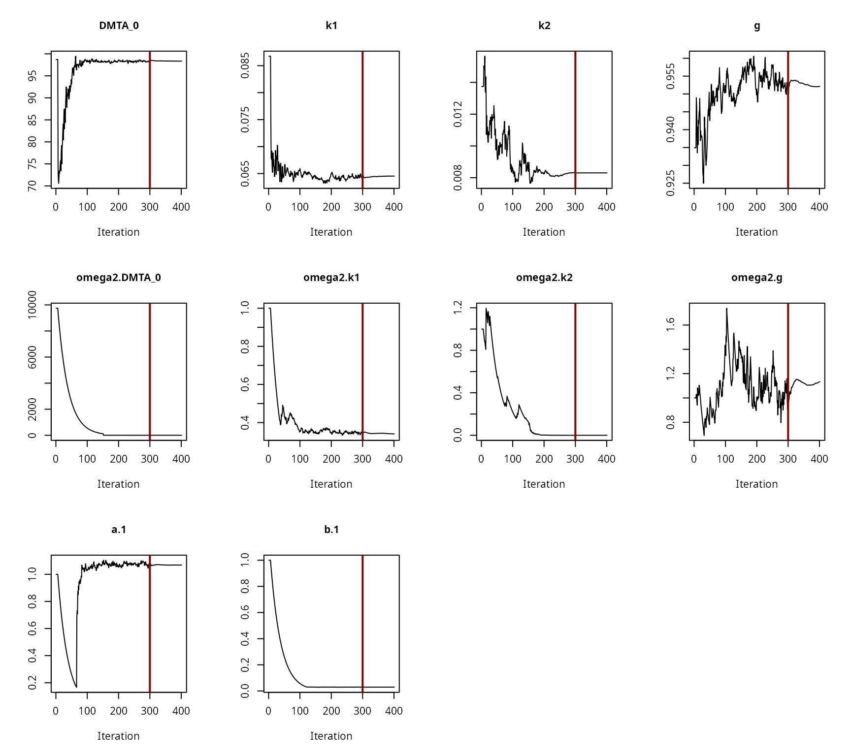
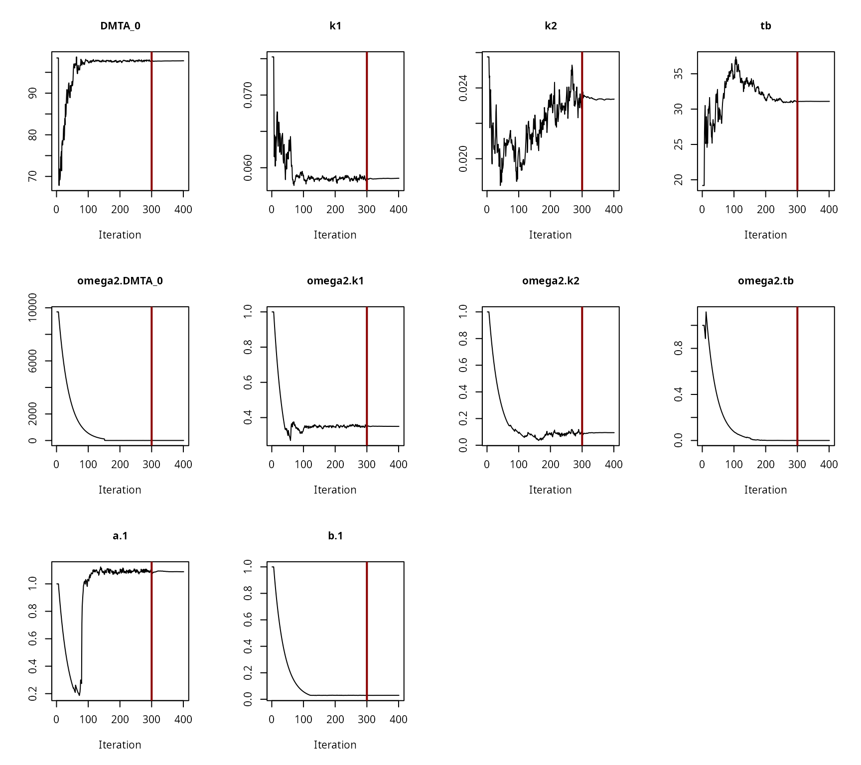
The convergence of the fit is checked visually.
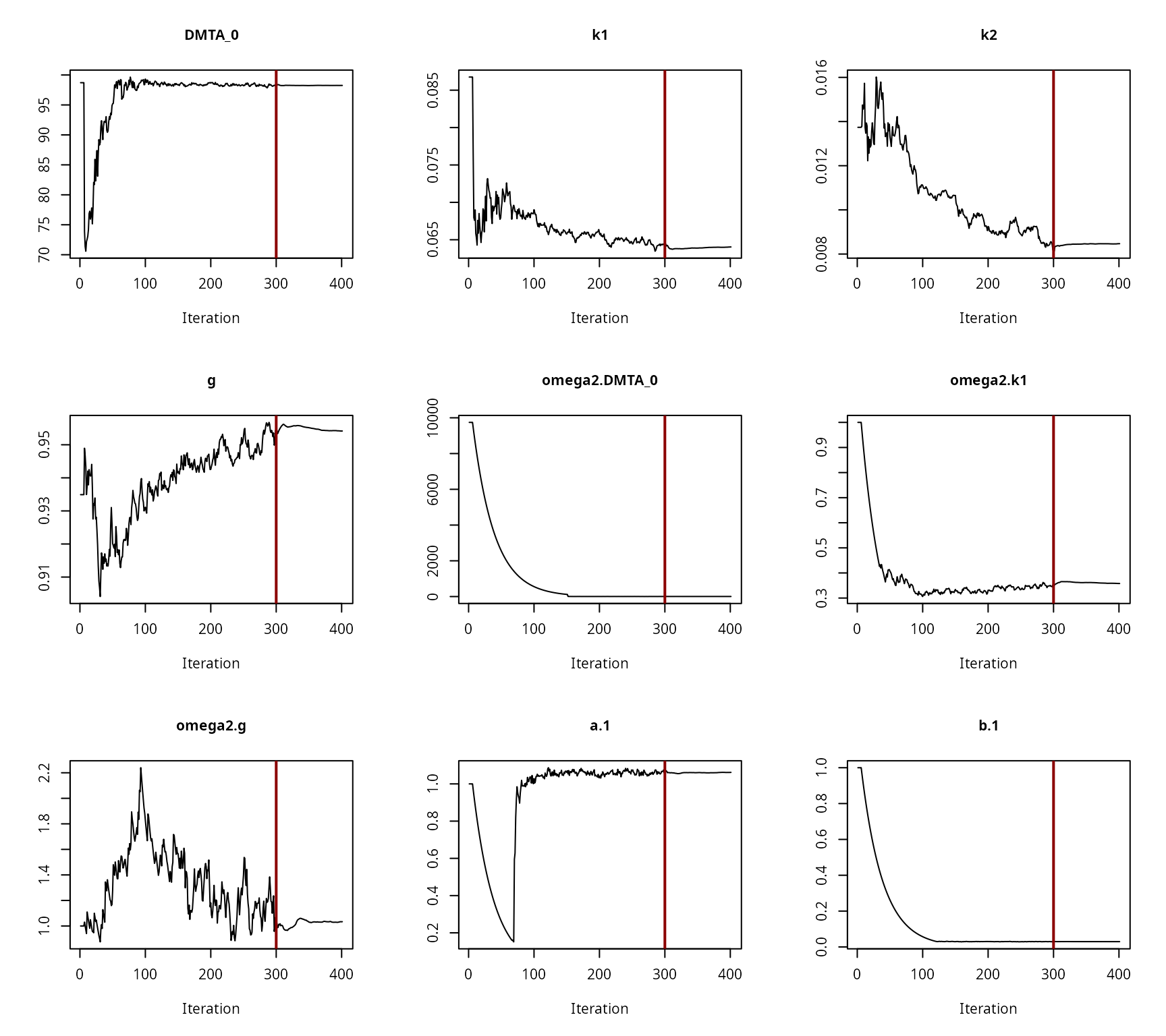
Convergence plot for the NLHM DFOP fit with two-component error and without a random effect on ‘k2’
All parameters appear to have converged to a satisfactory degree. The final fit is plotted using the plot method from the mkin package.
plot(f_saem_dfop_tc_no_ranef_k2)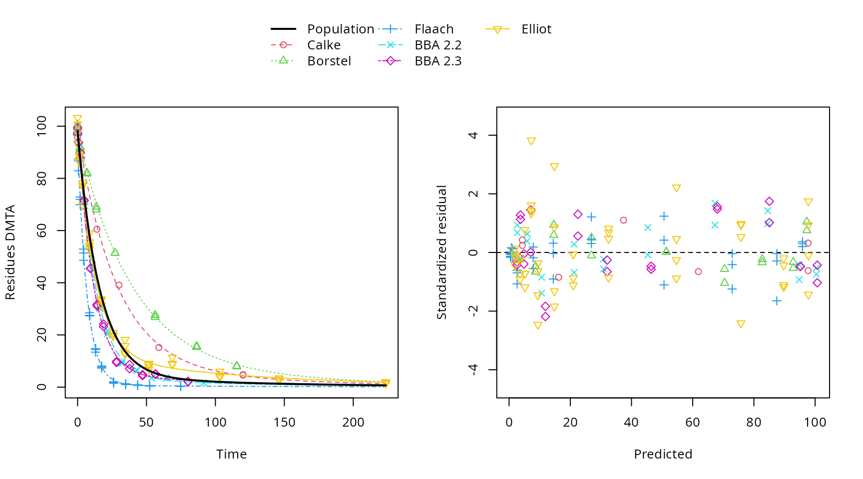
Plot of the final NLHM DFOP fit
Finally, a summary report of the fit is produced.
summary(f_saem_dfop_tc_no_ranef_k2)saemix version used for fitting: 3.3
mkin version used for pre-fitting: 1.2.10
R version used for fitting: 4.5.0
Date of fit: Mon May 12 21:06:46 2025
Date of summary: Mon May 12 21:06:46 2025
Equations:
d_DMTA/dt = - ((k1 * g * exp(-k1 * time) + k2 * (1 - g) * exp(-k2 *
time)) / (g * exp(-k1 * time) + (1 - g) * exp(-k2 * time)))
* DMTA
Data:
155 observations of 1 variable(s) grouped in 6 datasets
Model predictions using solution type analytical
Fitted in 3.953 s
Using 300, 100 iterations and 9 chains
Variance model: Two-component variance function
Starting values for degradation parameters:
DMTA_0 k1 k2 g
98.71186 0.08675 0.01374 0.93491
Fixed degradation parameter values:
None
Starting values for random effects (square root of initial entries in omega):
DMTA_0 k1 k2 g
DMTA_0 98.71 0 0 0
k1 0.00 1 0 0
k2 0.00 0 1 0
g 0.00 0 0 1
Starting values for error model parameters:
a.1 b.1
1 1
Results:
Likelihood computed by importance sampling
AIC BIC logLik
663.7 661.8 -322.9
Optimised parameters:
est. lower upper
DMTA_0 98.256267 96.286112 100.22642
k1 0.064037 0.033281 0.09479
k2 0.008469 0.006002 0.01094
g 0.954167 0.914460 0.99387
a.1 1.061795 0.878608 1.24498
b.1 0.029550 0.022593 0.03651
SD.DMTA_0 2.068581 0.427178 3.70998
SD.k1 0.598285 0.258235 0.93833
SD.g 1.016689 0.360061 1.67332
Correlation:
DMTA_0 k1 k2
k1 0.0213
k2 0.0541 0.0344
g -0.0521 -0.0286 -0.2744
Random effects:
est. lower upper
SD.DMTA_0 2.0686 0.4272 3.7100
SD.k1 0.5983 0.2582 0.9383
SD.g 1.0167 0.3601 1.6733
Variance model:
est. lower upper
a.1 1.06180 0.87861 1.24498
b.1 0.02955 0.02259 0.03651
Estimated disappearance times:
DT50 DT90 DT50back DT50_k1 DT50_k2
DMTA 11.45 41.32 12.44 10.82 81.85Alternative check of parameter identifiability
The parameter check used in the illparms function is
based on a quadratic approximation of the likelihood surface near its
optimum, which is calculated using the Fisher Information Matrix (FIM).
An alternative way to check parameter identifiability (Duchesne et al. 2021) based on a multistart
approach has recently been implemented in mkin.
The graph below shows boxplots of the parameters obtained in 50 runs of the saem algorithm with different parameter combinations, sampled from the range of the parameters obtained for the individual datasets fitted separately using nonlinear regression.
f_saem_dfop_tc_multi <- multistart(f_saem[["DFOP", "tc"]], n = 50, cores = 15)
par(mar = c(6.1, 4.1, 2.1, 2.1))
parplot(f_saem_dfop_tc_multi, lpos = "bottomright", ylim = c(0.3, 10), las = 2)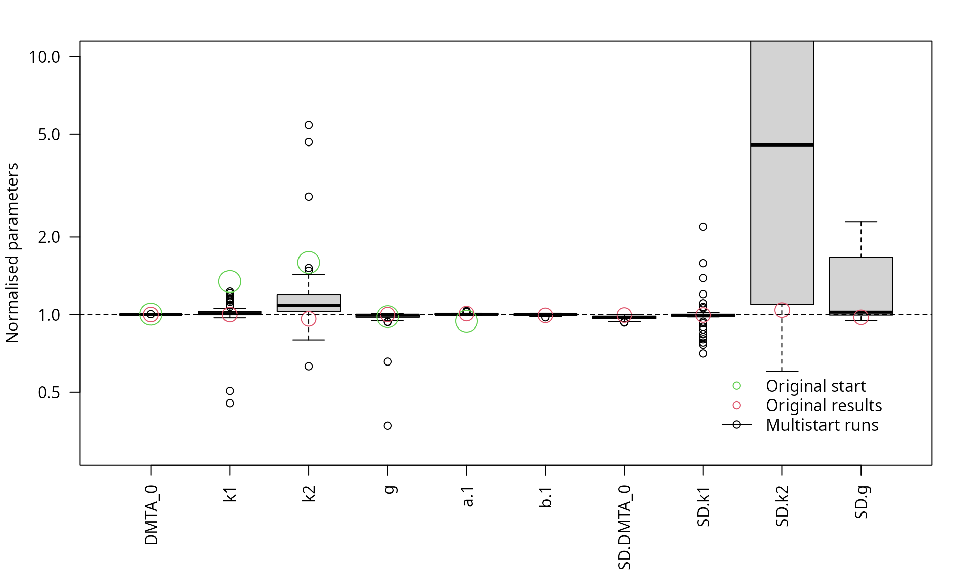
Scaled parameters from the multistart runs, full model
The graph clearly confirms the lack of identifiability of the
variance of k2 in the full model. The overparameterisation
of the model also indicates a lack of identifiability of the variance of
parameter g.
The parameter boxplots of the multistart runs with the reduced model shown below indicate that all runs give similar results, regardless of the starting parameters.
f_saem_dfop_tc_no_ranef_k2_multi <- multistart(f_saem_dfop_tc_no_ranef_k2,
  n = 50, cores = 15)
par(mar = c(6.1, 4.1, 2.1, 2.1))
parplot(f_saem_dfop_tc_no_ranef_k2_multi, ylim = c(0.5, 2), las = 2,
  lpos = "bottomright")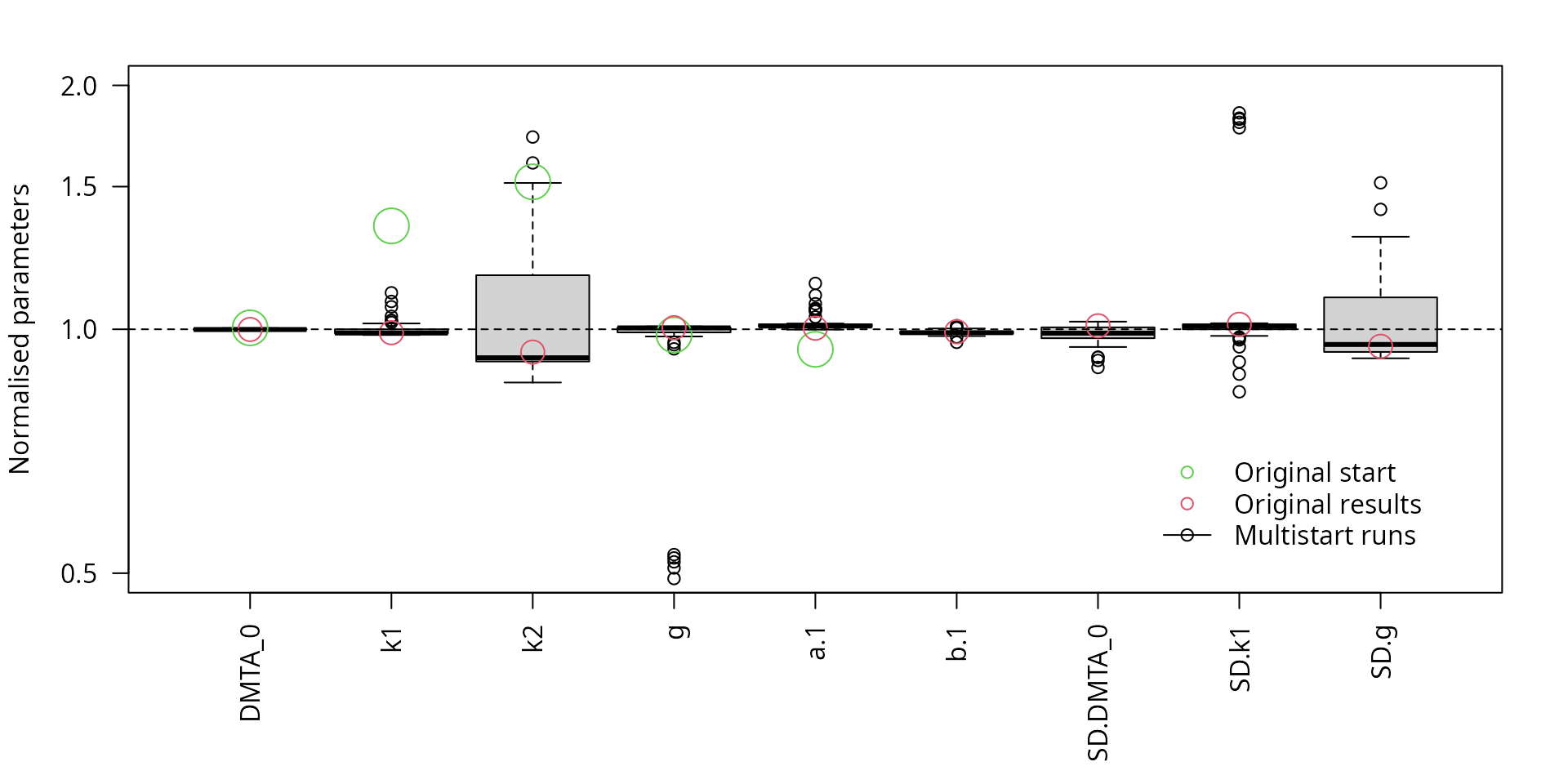
Scaled parameters from the multistart runs, reduced model
When only the parameters of the top 25% of the fits are shown (based on a feature introduced in mkin 1.2.2 currently under development), the scatter is even less as shown below.
par(mar = c(6.1, 4.1, 2.1, 2.1))
parplot(f_saem_dfop_tc_no_ranef_k2_multi, ylim = c(0.5, 2), las = 2, llquant = 0.25,
  lpos = "bottomright")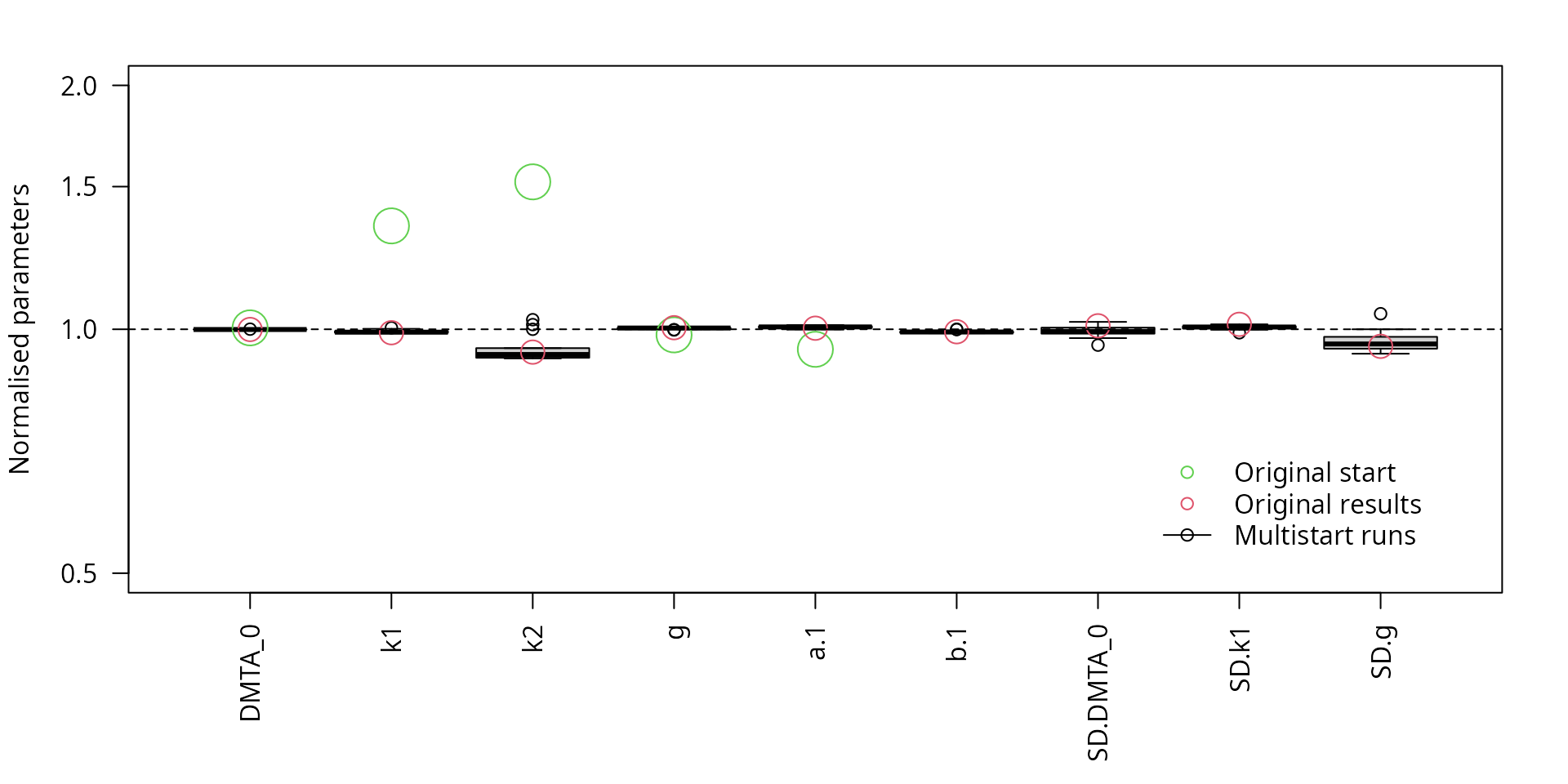
Scaled parameters from the multistart runs, reduced model, fits with the top 25% likelihood values
Conclusions
Fitting the four parent degradation models SFO, FOMC, DFOP and HS as part of hierarchical model fits with two different error models and normal distributions of the transformed degradation parameters works without technical problems. The biphasic models DFOP and HS gave the best fit to the data, but the default parameter distribution model was not fully identifiable. Removing the random effect for the second kinetic rate constant of the DFOP model resulted in a reduced model that was fully identifiable and showed the lowest values for the model selection criteria AIC and BIC. The reliability of the identification of all model parameters was confirmed using multiple starting values.
Acknowledgements
The helpful comments by Janina Wöltjen of the German Environment Agency are gratefully acknowledged.
References
Appendix
Hierarchical model fit listings
saemix version used for fitting:      3.3
mkin version used for pre-fitting:  1.2.10
R version used for fitting:         4.5.0
Date of fit:     Mon May 12 21:06:38 2025
Date of summary: Mon May 12 21:07:51 2025

Equations:
d_DMTA/dt = - k_DMTA * DMTA

Data:
155 observations of 1 variable(s) grouped in 6 datasets

Model predictions using solution type analytical

Fitted in 0.793 s
Using 300, 100 iterations and 9 chains

Variance model: Constant variance

Starting values for degradation parameters:
 DMTA_0  k_DMTA
97.2953  0.0566

Fixed degradation parameter values:
None

Starting values for random effects (square root of initial entries in omega):
       DMTA_0 k_DMTA
DMTA_0   97.3      0
k_DMTA    0.0      1

Starting values for error model parameters:
a.1
  1

Results:

Likelihood computed by importance sampling
    AIC   BIC logLik
  796.3 795.3 -393.2

Optimised parameters:
              est.    lower   upper
DMTA_0    97.28130 95.71113 98.8515
k_DMTA     0.05665  0.02909  0.0842
a.1        2.66442  2.35579  2.9731
SD.DMTA_0  1.54776  0.15447  2.9411
SD.k_DMTA  0.60690  0.26248  0.9513

Correlation:
       DMTA_0
k_DMTA 0.0168

Random effects:
            est.  lower  upper
SD.DMTA_0 1.5478 0.1545 2.9411
SD.k_DMTA 0.6069 0.2625 0.9513

Variance model:
     est. lower upper
a.1 2.664 2.356 2.973

Estimated disappearance times:
      DT50  DT90
DMTA 12.24 40.65
saemix version used for fitting:      3.3
mkin version used for pre-fitting:  1.2.10
R version used for fitting:         4.5.0
Date of fit:     Mon May 12 21:06:40 2025
Date of summary: Mon May 12 21:07:51 2025

Equations:
d_DMTA/dt = - k_DMTA * DMTA

Data:
155 observations of 1 variable(s) grouped in 6 datasets

Model predictions using solution type analytical

Fitted in 2.462 s
Using 300, 100 iterations and 9 chains

Variance model: Two-component variance function

Starting values for degradation parameters:
  DMTA_0   k_DMTA
96.99175  0.05603

Fixed degradation parameter values:
None

Starting values for random effects (square root of initial entries in omega):
       DMTA_0 k_DMTA
DMTA_0  96.99      0
k_DMTA   0.00      1

Starting values for error model parameters:
a.1 b.1
  1   1

Results:

Likelihood computed by importance sampling
    AIC   BIC logLik
  798.3 797.1 -393.2

Optimised parameters:
               est.    lower    upper
DMTA_0    97.271822 95.70316 98.84049
k_DMTA     0.056638  0.02911  0.08417
a.1        2.660081  2.27492  3.04525
b.1        0.001665 -0.14451  0.14784
SD.DMTA_0  1.545520  0.14301  2.94803
SD.k_DMTA  0.606422  0.26227  0.95057

Correlation:
       DMTA_0
k_DMTA 0.0169

Random effects:
            est.  lower  upper
SD.DMTA_0 1.5455 0.1430 2.9480
SD.k_DMTA 0.6064 0.2623 0.9506

Variance model:
        est.   lower  upper
a.1 2.660081  2.2749 3.0452
b.1 0.001665 -0.1445 0.1478

Estimated disappearance times:
      DT50  DT90
DMTA 12.24 40.65
saemix version used for fitting:      3.3
mkin version used for pre-fitting:  1.2.10
R version used for fitting:         4.5.0
Date of fit:     Mon May 12 21:06:39 2025
Date of summary: Mon May 12 21:07:51 2025

Equations:
d_DMTA/dt = - (alpha/beta) * 1/((time/beta) + 1) * DMTA

Data:
155 observations of 1 variable(s) grouped in 6 datasets

Model predictions using solution type analytical

Fitted in 1.408 s
Using 300, 100 iterations and 9 chains

Variance model: Constant variance

Starting values for degradation parameters:
 DMTA_0   alpha    beta
 98.292   9.909 156.341

Fixed degradation parameter values:
None

Starting values for random effects (square root of initial entries in omega):
       DMTA_0 alpha beta
DMTA_0  98.29     0    0
alpha    0.00     1    0
beta     0.00     0    1

Starting values for error model parameters:
a.1
  1

Results:

Likelihood computed by importance sampling
    AIC   BIC logLik
  734.2 732.7 -360.1

Optimised parameters:
              est.   lower   upper
DMTA_0     98.3435 96.9033  99.784
alpha       7.2007  2.5889  11.812
beta      112.8745 34.8816 190.867
a.1         2.0459  1.8054   2.286
SD.DMTA_0   1.4795  0.2717   2.687
SD.alpha    0.6396  0.1509   1.128
SD.beta     0.6874  0.1587   1.216

Correlation:
      DMTA_0  alpha
alpha -0.1125
beta  -0.1227  0.3632

Random effects:
            est.  lower upper
SD.DMTA_0 1.4795 0.2717 2.687
SD.alpha  0.6396 0.1509 1.128
SD.beta   0.6874 0.1587 1.216

Variance model:
     est. lower upper
a.1 2.046 1.805 2.286

Estimated disappearance times:
      DT50  DT90 DT50back
DMTA 11.41 42.53     12.8
saemix version used for fitting:      3.3
mkin version used for pre-fitting:  1.2.10
R version used for fitting:         4.5.0
Date of fit:     Mon May 12 21:06:40 2025
Date of summary: Mon May 12 21:07:51 2025

Equations:
d_DMTA/dt = - (alpha/beta) * 1/((time/beta) + 1) * DMTA

Data:
155 observations of 1 variable(s) grouped in 6 datasets

Model predictions using solution type analytical

Fitted in 2.735 s
Using 300, 100 iterations and 9 chains

Variance model: Two-component variance function

Starting values for degradation parameters:
DMTA_0  alpha   beta
98.772  4.663 92.597

Fixed degradation parameter values:
None

Starting values for random effects (square root of initial entries in omega):
       DMTA_0 alpha beta
DMTA_0  98.77     0    0
alpha    0.00     1    0
beta     0.00     0    1

Starting values for error model parameters:
a.1 b.1
  1   1

Results:

Likelihood computed by importance sampling
    AIC   BIC logLik
  720.7 719.1 -352.4

Optimised parameters:
              est.    lower     upper
DMTA_0    99.10577 97.33296 100.87859
alpha      5.46260  2.52199   8.40321
beta      81.66080 30.46664 132.85497
a.1        1.50219  1.25801   1.74636
b.1        0.02893  0.02048   0.03739
SD.DMTA_0  1.61887 -0.03843   3.27618
SD.alpha   0.58145  0.17364   0.98925
SD.beta    0.68205  0.21108   1.15302

Correlation:
      DMTA_0  alpha
alpha -0.1321
beta  -0.1430  0.2467

Random effects:
            est.    lower  upper
SD.DMTA_0 1.6189 -0.03843 3.2762
SD.alpha  0.5814  0.17364 0.9892
SD.beta   0.6821  0.21108 1.1530

Variance model:
       est.   lower   upper
a.1 1.50219 1.25801 1.74636
b.1 0.02893 0.02048 0.03739

Estimated disappearance times:
      DT50  DT90 DT50back
DMTA 11.05 42.81    12.89
saemix version used for fitting:      3.3
mkin version used for pre-fitting:  1.2.10
R version used for fitting:         4.5.0
Date of fit:     Mon May 12 21:06:39 2025
Date of summary: Mon May 12 21:07:51 2025

Equations:
d_DMTA/dt = - ((k1 * g * exp(-k1 * time) + k2 * (1 - g) * exp(-k2 *
           time)) / (g * exp(-k1 * time) + (1 - g) * exp(-k2 * time)))
           * DMTA

Data:
155 observations of 1 variable(s) grouped in 6 datasets

Model predictions using solution type analytical

Fitted in 1.769 s
Using 300, 100 iterations and 9 chains

Variance model: Constant variance

Starting values for degradation parameters:
  DMTA_0       k1       k2        g
98.64383  0.09211  0.02999  0.76814

Fixed degradation parameter values:
None

Starting values for random effects (square root of initial entries in omega):
       DMTA_0 k1 k2 g
DMTA_0  98.64  0  0 0
k1       0.00  1  0 0
k2       0.00  0  1 0
g        0.00  0  0 1

Starting values for error model parameters:
a.1
  1

Results:

Likelihood computed by importance sampling
    AIC BIC logLik
  711.8 710 -346.9

Optimised parameters:
               est.     lower    upper
DMTA_0    98.092481 96.573899 99.61106
k1         0.062499  0.030336  0.09466
k2         0.009065 -0.005133  0.02326
g          0.948967  0.862080  1.03586
a.1        1.821671  1.604774  2.03857
SD.DMTA_0  1.677785  0.472066  2.88350
SD.k1      0.634962  0.270788  0.99914
SD.k2      1.033498 -0.205994  2.27299
SD.g       1.710046  0.428642  2.99145

Correlation:
   DMTA_0  k1      k2
k1  0.0246
k2  0.0491  0.0953
g  -0.0552 -0.0889 -0.4795

Random effects:
           est.   lower  upper
SD.DMTA_0 1.678  0.4721 2.8835
SD.k1     0.635  0.2708 0.9991
SD.k2     1.033 -0.2060 2.2730
SD.g      1.710  0.4286 2.9914

Variance model:
     est. lower upper
a.1 1.822 1.605 2.039

Estimated disappearance times:
      DT50 DT90 DT50back DT50_k1 DT50_k2
DMTA 11.79 42.8    12.88   11.09   76.46
saemix version used for fitting:      3.3
mkin version used for pre-fitting:  1.2.10
R version used for fitting:         4.5.0
Date of fit:     Mon May 12 21:06:41 2025
Date of summary: Mon May 12 21:07:51 2025

Equations:
d_DMTA/dt = - ((k1 * g * exp(-k1 * time) + k2 * (1 - g) * exp(-k2 *
           time)) / (g * exp(-k1 * time) + (1 - g) * exp(-k2 * time)))
           * DMTA

Data:
155 observations of 1 variable(s) grouped in 6 datasets

Model predictions using solution type analytical

Fitted in 3.069 s
Using 300, 100 iterations and 9 chains

Variance model: Two-component variance function

Starting values for degradation parameters:
  DMTA_0       k1       k2        g
98.71186  0.08675  0.01374  0.93491

Fixed degradation parameter values:
None

Starting values for random effects (square root of initial entries in omega):
       DMTA_0 k1 k2 g
DMTA_0  98.71  0  0 0
k1       0.00  1  0 0
k2       0.00  0  1 0
g        0.00  0  0 1

Starting values for error model parameters:
a.1 b.1
  1   1

Results:

Likelihood computed by importance sampling
    AIC   BIC logLik
  665.7 663.6 -322.9

Optimised parameters:
               est.     lower     upper
DMTA_0    98.347470 96.380815 100.31413
k1         0.064524  0.034279   0.09477
k2         0.008304  0.005843   0.01076
g          0.952128  0.909578   0.99468
a.1        1.068907  0.883665   1.25415
b.1        0.029265  0.022318   0.03621
SD.DMTA_0  2.065796  0.427951   3.70364
SD.k1      0.583703  0.251796   0.91561
SD.k2      0.004167 -7.831228   7.83956
SD.g       1.064450  0.397479   1.73142

Correlation:
   DMTA_0  k1      k2
k1  0.0223
k2  0.0568  0.0394
g  -0.0464 -0.0269 -0.2713

Random effects:
              est.   lower  upper
SD.DMTA_0 2.065796  0.4280 3.7036
SD.k1     0.583703  0.2518 0.9156
SD.k2     0.004167 -7.8312 7.8396
SD.g      1.064450  0.3975 1.7314

Variance model:
       est.   lower   upper
a.1 1.06891 0.88367 1.25415
b.1 0.02927 0.02232 0.03621

Estimated disappearance times:
      DT50  DT90 DT50back DT50_k1 DT50_k2
DMTA 11.39 41.36    12.45   10.74   83.48
saemix version used for fitting:      3.3
mkin version used for pre-fitting:  1.2.10
R version used for fitting:         4.5.0
Date of fit:     Mon May 12 21:06:39 2025
Date of summary: Mon May 12 21:07:51 2025

Equations:
d_DMTA/dt = - ifelse(time <= tb, k1, k2) * DMTA

Data:
155 observations of 1 variable(s) grouped in 6 datasets

Model predictions using solution type analytical

Fitted in 1.996 s
Using 300, 100 iterations and 9 chains

Variance model: Constant variance

Starting values for degradation parameters:
  DMTA_0       k1       k2       tb
97.82176  0.06931  0.02997 11.13945

Fixed degradation parameter values:
None

Starting values for random effects (square root of initial entries in omega):
       DMTA_0 k1 k2 tb
DMTA_0  97.82  0  0  0
k1       0.00  1  0  0
k2       0.00  0  1  0
tb       0.00  0  0  1

Starting values for error model parameters:
a.1
  1

Results:

Likelihood computed by importance sampling
  AIC   BIC logLik
  714 712.1   -348

Optimised parameters:
              est.    lower    upper
DMTA_0    98.16102 96.47747 99.84456
k1         0.07876  0.05261  0.10491
k2         0.02227  0.01706  0.02747
tb        13.99089 -7.40049 35.38228
a.1        1.82305  1.60700  2.03910
SD.DMTA_0  1.88413  0.56204  3.20622
SD.k1      0.34292  0.10482  0.58102
SD.k2      0.19851  0.01718  0.37985
SD.tb      1.68168  0.58064  2.78272

Correlation:
   DMTA_0  k1      k2
k1  0.0142
k2  0.0001 -0.0025
tb  0.0165 -0.1256 -0.0301

Random effects:
            est.   lower  upper
SD.DMTA_0 1.8841 0.56204 3.2062
SD.k1     0.3429 0.10482 0.5810
SD.k2     0.1985 0.01718 0.3798
SD.tb     1.6817 0.58064 2.7827

Variance model:
     est. lower upper
a.1 1.823 1.607 2.039

Estimated disappearance times:
      DT50  DT90 DT50back DT50_k1 DT50_k2
DMTA 8.801 67.91    20.44   8.801   31.13
saemix version used for fitting:      3.3
mkin version used for pre-fitting:  1.2.10
R version used for fitting:         4.5.0
Date of fit:     Mon May 12 21:06:41 2025
Date of summary: Mon May 12 21:07:51 2025

Equations:
d_DMTA/dt = - ifelse(time <= tb, k1, k2) * DMTA

Data:
155 observations of 1 variable(s) grouped in 6 datasets

Model predictions using solution type analytical

Fitted in 3.389 s
Using 300, 100 iterations and 9 chains

Variance model: Two-component variance function

Starting values for degradation parameters:
  DMTA_0       k1       k2       tb
98.45190  0.07525  0.02576 19.19375

Fixed degradation parameter values:
None

Starting values for random effects (square root of initial entries in omega):
       DMTA_0 k1 k2 tb
DMTA_0  98.45  0  0  0
k1       0.00  1  0  0
k2       0.00  0  1  0
tb       0.00  0  0  1

Starting values for error model parameters:
a.1 b.1
  1   1

Results:

Likelihood computed by importance sampling
    AIC BIC logLik
  667.1 665 -323.6

Optimised parameters:
              est.    lower    upper
DMTA_0    97.76571 95.81350 99.71791
k1         0.05855  0.03080  0.08630
k2         0.02337  0.01664  0.03010
tb        31.09638 29.38289 32.80987
a.1        1.08835  0.90059  1.27611
b.1        0.02964  0.02261  0.03667
SD.DMTA_0  2.04877  0.42553  3.67200
SD.k1      0.59166  0.25621  0.92711
SD.k2      0.30698  0.09561  0.51835
SD.tb      0.01274 -0.10915  0.13464

Correlation:
   DMTA_0  k1      k2
k1  0.0160
k2 -0.0070 -0.0024
tb -0.0668 -0.0103 -0.2013

Random effects:
             est.    lower  upper
SD.DMTA_0 2.04877  0.42553 3.6720
SD.k1     0.59166  0.25621 0.9271
SD.k2     0.30698  0.09561 0.5183
SD.tb     0.01274 -0.10915 0.1346

Variance model:
       est.   lower   upper
a.1 1.08835 0.90059 1.27611
b.1 0.02964 0.02261 0.03667

Estimated disappearance times:
      DT50  DT90 DT50back DT50_k1 DT50_k2
DMTA 11.84 51.71    15.57   11.84   29.66
Hierarchical model convergence plots
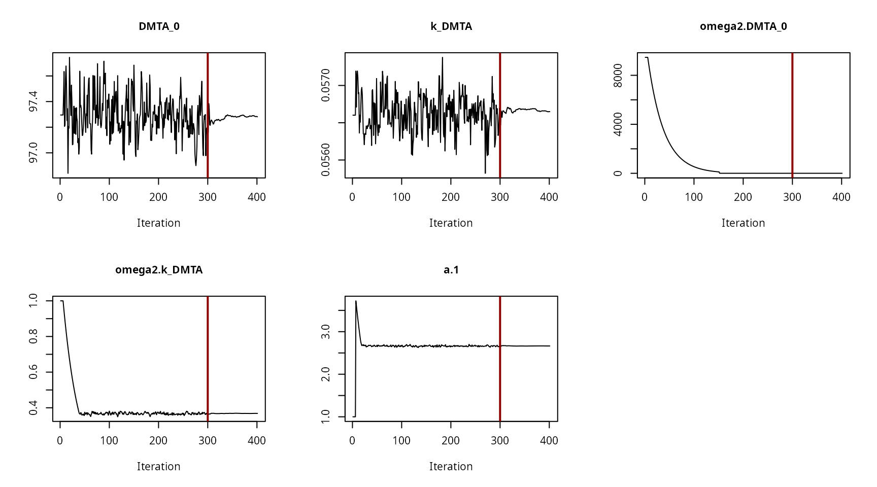
Convergence plot for the NLHM SFO fit with constant variance
Convergence plot for the NLHM SFO fit with two-component error
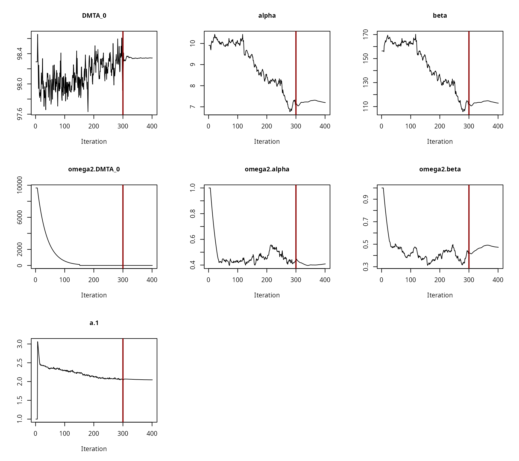
Convergence plot for the NLHM FOMC fit with constant variance
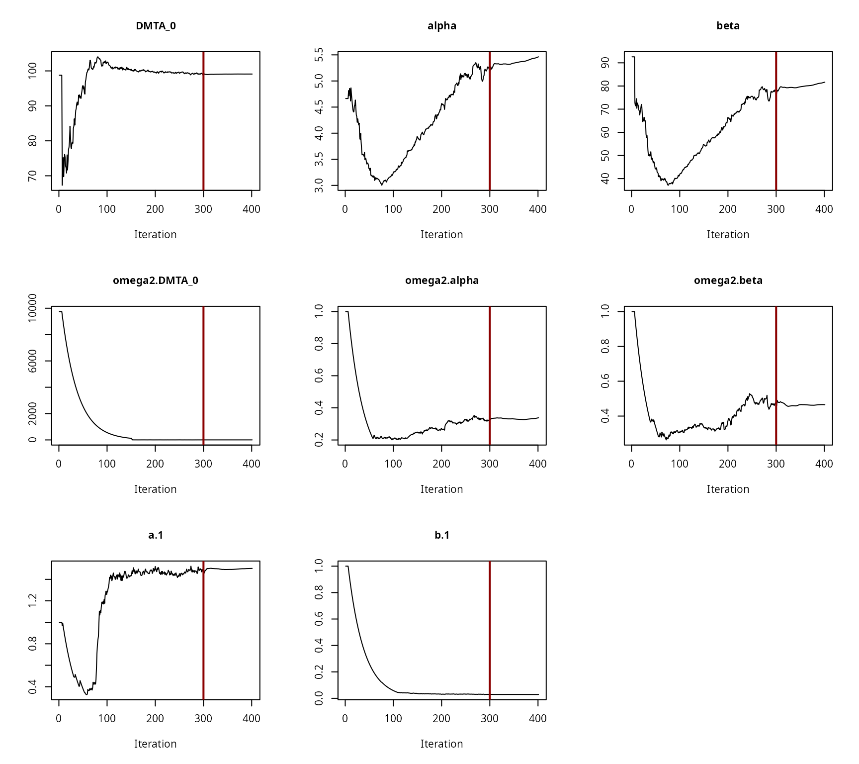
Convergence plot for the NLHM FOMC fit with two-component error
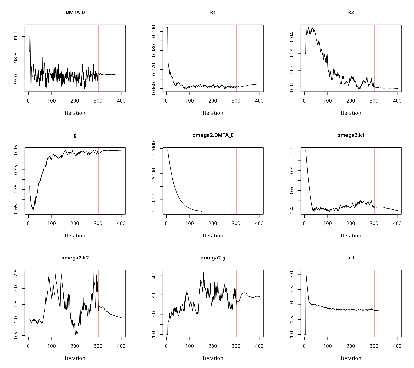
Convergence plot for the NLHM DFOP fit with constant variance
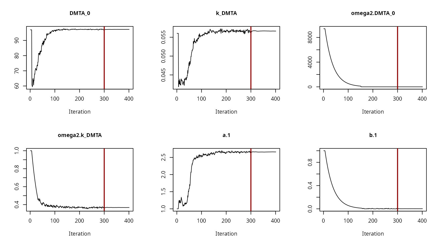
Convergence plot for the NLHM DFOP fit with two-component error
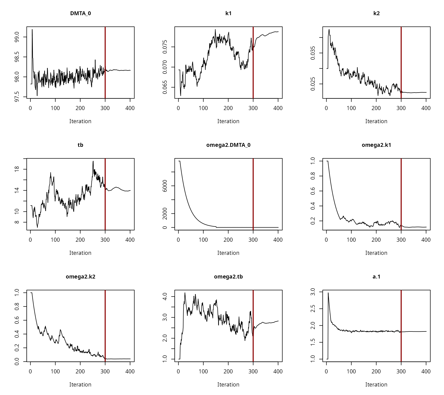
Convergence plot for the NLHM HS fit with constant variance
Convergence plot for the NLHM HS fit with two-component error
Session info
R version 4.5.0 (2025-04-11)
Platform: x86_64-pc-linux-gnu
Running under: Debian GNU/Linux 12 (bookworm)

Matrix products: default
BLAS:   /usr/lib/x86_64-linux-gnu/blas/libblas.so.3.11.0
LAPACK: /usr/lib/x86_64-linux-gnu/lapack/liblapack.so.3.11.0  LAPACK version 3.11.0

locale:
 [1] LC_CTYPE=de_DE.UTF-8       LC_NUMERIC=C
 [3] LC_TIME=de_DE.UTF-8        LC_COLLATE=de_DE.UTF-8
 [5] LC_MONETARY=de_DE.UTF-8    LC_MESSAGES=de_DE.UTF-8
 [7] LC_PAPER=de_DE.UTF-8       LC_NAME=C
 [9] LC_ADDRESS=C               LC_TELEPHONE=C
[11] LC_MEASUREMENT=de_DE.UTF-8 LC_IDENTIFICATION=C

time zone: Europe/Berlin
tzcode source: system (glibc)

attached base packages:
[1] parallel  stats     graphics  grDevices utils     datasets  methods
[8] base

other attached packages:
[1] rmarkdown_2.29  nvimcom_0.9-167 saemix_3.3      npde_3.5
[5] knitr_1.49      mkin_1.2.10

loaded via a namespace (and not attached):
 [1] gtable_0.3.6      jsonlite_1.9.0    dplyr_1.1.4       compiler_4.5.0
 [5] tidyselect_1.2.1  gridExtra_2.3     jquerylib_0.1.4   systemfonts_1.2.1
 [9] scales_1.3.0      textshaping_1.0.0 yaml_2.3.10       fastmap_1.2.0
[13] lattice_0.22-6    ggplot2_3.5.1     R6_2.6.1          generics_0.1.3
[17] lmtest_0.9-40     MASS_7.3-65       htmlwidgets_1.6.4 tibble_3.2.1
[21] desc_1.4.3        munsell_0.5.1     bslib_0.9.0       pillar_1.10.1
[25] rlang_1.1.5       cachem_1.1.0      xfun_0.51         fs_1.6.5
[29] sass_0.4.9        cli_3.6.4         pkgdown_2.1.1     magrittr_2.0.3
[33] digest_0.6.37     grid_4.5.0        mclust_6.1.1      lifecycle_1.0.4
[37] nlme_3.1-168      vctrs_0.6.5       evaluate_1.0.3    glue_1.8.0
[41] codetools_0.2-20  ragg_1.3.3        zoo_1.8-13        colorspace_2.1-1
[45] tools_4.5.0       pkgconfig_2.0.3   htmltools_0.5.8.1